Creating Charts in Excel is very easy, we change the look and feel by working with Chart Styles Layouts and Templates in Excel. Chart Styles, Layouts and Templates in Excel help us to change the look and feel of the charts to create rich visualized charts in excel for your data.
Working with Styles in Excel
Once your are done with the creating chart in Excel, you can then change the look and feel of the chart. There are many predefined styles available in Excel, you can simply select and change the Chart Styles.
What are Chart Styles in Excel?
Chart Styles in Excel are predefined styles which can be applied to your charts to quickly change its look and feel.
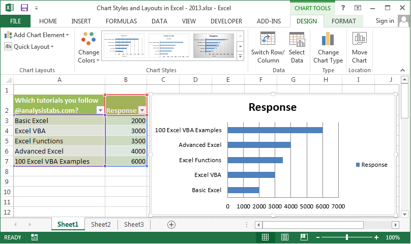
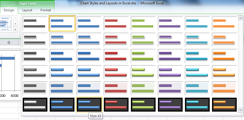
I have create an Example Chart with some random data. When you select your chart you can observe the Style are available in the design Tab of the Excel ribbon.
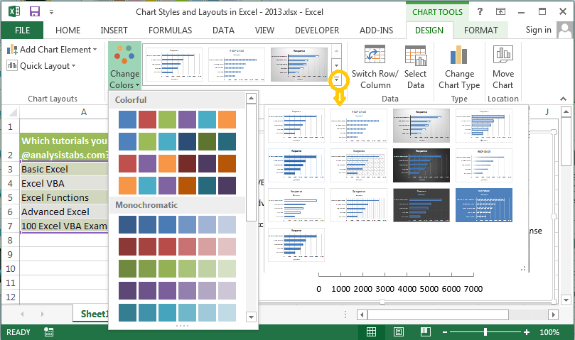
To view more styles, you can click on the scroll bar at right side of the styles.
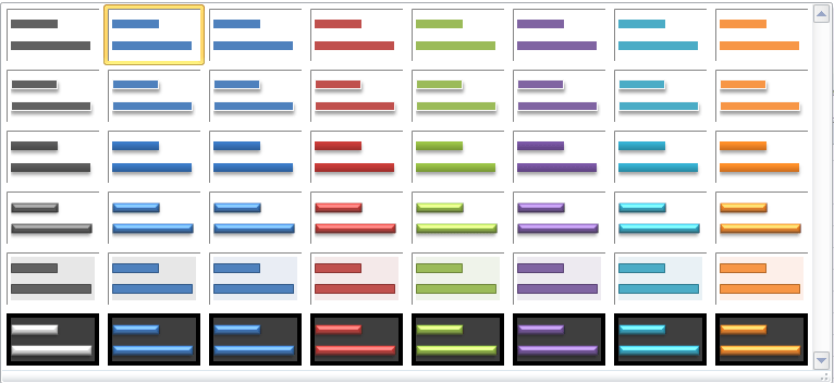
Following are the Styles in Design tab Excel 2013 Ribbon Menu.
Practical Learning – Applying Chart Styles in Excel
Now we will see how to change the styles step by step: These steps are more or less same in Excel 2007,Excel 2010 and Excel 2013.
Step 1: Select a Chart to change its styles: First you need to select a chart which you would like to change its style.
Step 2: Go to Design Tab in Excel Ribbon: When you select the Chart you can see the design tab under Chart Tools in the Excel Ribbon. And can see the styles menu group in the Design Ribbon.
Step 3: Select a style from the Chart Styles menu tab: Now you can select the desired style from the Styles available in the Styles group. If you want to see more styles, you can click on the scroll bar at right side of the styles, then select desired Chart style to apply.
Working with Layouts in Excel
Chart styles are particularly for styling and changing the look and feel of the charts. Layouts will provide more chart elements to understand the charts better.
What are Chart Layouts in Excel?
Chart Layouts in Excel are predefined Chart Layouts to add more chart elements in Excel Charts to increase the readbility for better understanding the Charts.
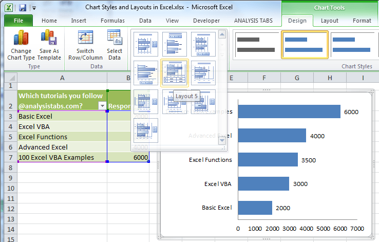
For example, If you want to see the chart data table on your chart you can goto Chart Layouts and Apply the Chart Layout with Table. So many predefined chart layouts are available to add or remove the Data Tables, Legened, Titles and Gridlines,etc.
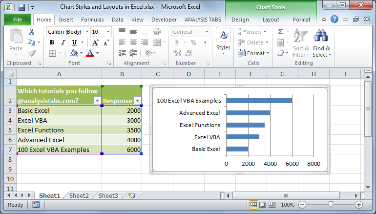
I am using the same chart created in above to expalin the Chart Layouts. When you select your chart you can observe the Chart Layouts are available in the design Tab of the Excel ribbon. Also a seperate tabe as Layout in Excel 2007 and 2010. In 2013 you will find these options as ‘Add Chart Elements’ and ‘Quick Layout’ ribbon menus in the Design Tab.
You can click on the scroll bar at right side of the Layout to view more Chart Layouts.
Practical Learning – Applying Chart Layouts in Excel
Followung are the steps to be followed for applying chart layouts in Excel: These steps are more or less same in Excel 2007,Excel 2010 and Excel 2013.
Step 1: Select a Chart to change its Layouts: First you need to select a chart which you would like to change its Layouts.
Step 2: Go to Design Tab in Excel Ribbon: When you select the Chart you can see the design tab under Chart Tools in the Excel Ribbon. And you can see the layouts menu group in the Design Ribbon.
Step 3: Select a style from the Chart Layouts menu: Now you can select the desired style from the Chart Layouts available in the Layouts group. If you want to see more Layouts, you can click on the scroll bar at right side of the styles, then select desired Chart Layout to apply.
Working with Templates in Excel
Now we will see the Chart Templates in Excel to fasten the Charting Tasks.
What are Chart Templates in Excel?
Chart Templates in Excel helps us to save a particular charts with desired styles and layouts. We can apply the chart template to achieve same type of the charts in the future.
For example, if you want to create same type of the charts with same styles and layouts. You can create charts with desired styles and layouts and save as chart template. And apply the same chart template for the remaining chart, it will save your time and fasten your charting task. You can maintain the same standards across the charts in your Workbook by using Chart templates.
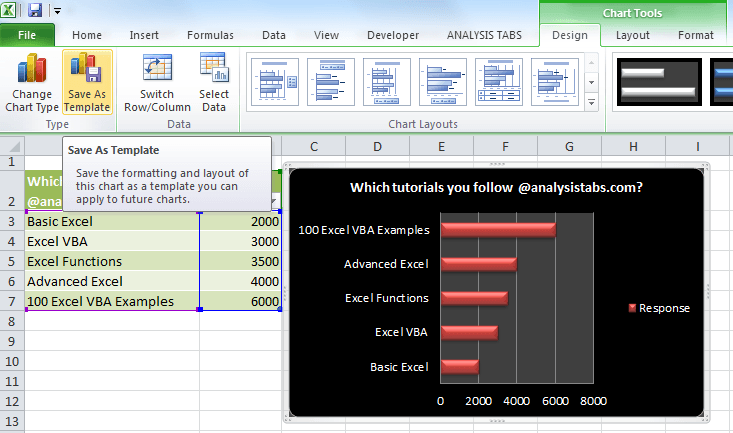
I have created a chart and changed its Chart Styles at Chart Layouts as shown below, I will use this chart to Explain Chart Templates in Excel.
Practical Learning – Applying Chart Templates in Excel
Following are the steps to be followed for saving and applying chart Templates in Excel: These steps are more or less same in Excel 2007,Excel 2010 and Excel 2013.
Step 1: Save your Chart as a Template: First you need to Save your chart in the Chart Templates after applying the Styels, Formats and Layouts.
1. Select your Chart which you want to save as Chart Template.
2. Go to Design Tab and Click on the Save Template button in the Type group in the ribbon.
In Excel 2013, you can right click on a Chart to add in to Templates and click on ‘Save as Template’
3. And Provide a Name for your Chart Template (I am giving ‘test’ in this example)
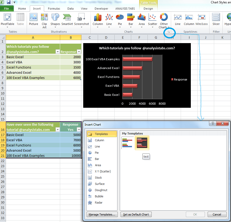
Step 2: Select Chart Data to Apply Chart Template: Now your chart template is ready and you can select your chart data to create the same type of chart.
Step 4: Select a style from the Chart Templates menu: Now you can select the desired Chart templates from your Saved Chart Templates available in the Chart Wizard.
1. Select your data to create New chart
2. Go to Insert Menu and Open the Chart Wizard
3. Select your chart template from the Templates available in the Chart Wizard
4. Then Click on OK button.
Now you can see a new chart is created as per your chart template:

