HLOOKUP Function in Excel – Formula Explained with Examples

What is the use of HLOOKUP function?

HLOOKUP is helpful to get the values from the lookup range, it search from top to bottom in Horizontal approach. VLOOKUP is useful for getting the data for lookup values by searching vertically. whare as HLOOKUP searches in Horizontally.

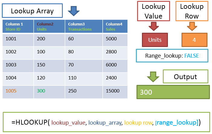
H in HLOOKUP stands for Horizoantal and HLOOKUP Function in Excel searches horizontally for lookup value and returns the value in a given row ( as per row index mentioned in the formula) that matches a value in the top most row of a table.

What is the syntax of HLOOKUP function?

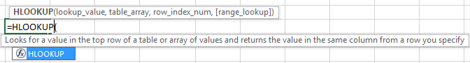
=HLOOKUP(lookup_value, table_array, row_index_num

• lookup_value: The value to be searched in the top most row of the array.
• table_array: The range or a range name containing the table of data.
• row_index_num: The row number in table_array from which you return corresponding matching value
  [range_lookup]: Whether to find an exact match.
  True or 1 = Closest match is returned
  False or 0 = Exact matches are returned

Examples on HLOOKUP Function in Excel

Let us see some examples to understand HLOOKUP formula.

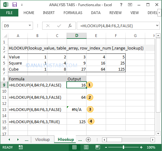
The data shows Square and Cube values in the rows for the columns 1 to 5.

Example 1:

=HLOOKUP(4,B4:F6,2,FALSE)

HLOOKUP Looks for the lookup value (4) in the top most row of the lookup range (first row, ie; B4:F4) and returns its corresponding value in the second row (as we mentioned row index as 2 in the HLOOKUP formula). So the result will be 16 (value found at 4th column, 2nd row)

Example 2:

=HLOOKUP(4,B4:F6,3,FALSE)

HLOOKUP Looks for the lookup value (4) in the top most row of the lookup range (first row, ie; B4:F4) and returns its corresponding value in the third row (as we mentioned row index as 3 in the HLOOKUP formula). So the result will be 64 (value found at 4th column, 3rd row)

Example 3:

=HLOOKUP(6,B4:F6,3,FALSE)

HLOOKUP Looks for the lookup value (6) in the top most row of the lookup range (first row, ie; B4:F4) and it should return its corresponding value in the third row (as we mentioned row index as 3 in the HLOOKUP formula).

This formula returns #NA as it does not found any match for lookup value in the lookup range (6 not found in in the table array or range B4:F4 ).

Example 4:

=HLOOKUP(6,B4:F6,3,TRUE)

HLOOKUP Looks for the lookup value (6) in the top most row of the lookup range (first row, ie; B4:F4) and it should return its corresponding value in the third row (as we mentioned row index as 3 in the HLOOKUP formula).

HLOOKUP returns 125 as 6 is not found in the lookup array (first row, ie; B4:F4) and we mentioned TRUE as match range type in the formula, So HLOOKUP wil search for nearest lookup value. 5 is closer to 6 and it returns its corresponding value in the third row i.e; 125.

Reference:

Please refer the below article for more Lookup & Reference Excel functions.
Lookup & Reference Excel Formulas

Please refer the below article for more Excel Functions.
Excel Formulas | Home