Yes, we can make Dynamic Chart Title by Linking and Reference to a Cell in Excel. This very useful when you want to change your chart title automatically when there is any change in data. Or else you can simply change the title in Cell or Range in the worksheet. You can link the Cell Reference or Range Address to chart title. Here is the simple practical example to show you how to link cell of worksheet to Chart title. We can also change the chart title based on the condition or formula by linking a Cell to the Chart. Even we can link a pivot table filter range to the chart title.
Dynamic Chart Title by Linking and Reference to a Cell in Excel – Practical Example
The following step by step approach is to show you example on Dynamic Chart Title by Linking and Reference to a Cell in Excel.
Linking Cell to make Dynamic Chart Title – Step 1: Select a Chart Title
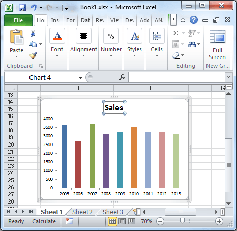
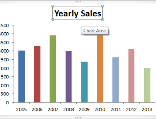
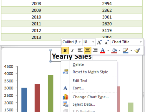
Identify the chart to link a cell reference to the chart title. The following screen-shot will show you example chart title is selected.
Here you can clearly observe that there is no formula is associated to chart title. You can observe that the address bar is empty.
Linking Cell to make Dynamic Chart Title – Step 2: Enter Cell Reference using Address bar
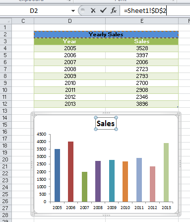
Go to the Address bar and type “=” and select a Cell to link. In the following example, we are linking the Cell D2.
Linking Cell to make Dynamic Chart Title – Step 3: Press Enter button to see the title
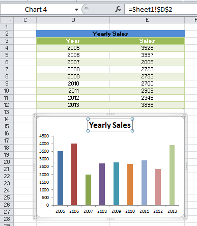
Once you are done with the linking, press the ‘Enter’ key to link the chart title to the Cell. Now you should able to see the chart title as specified in the Cell or Range D2 in the worksheet. This is the easiest approach to create Dynamic Chart Title by Linking and Reference to a Cell in Excel.
Changing the Chart title based on the Conditions
The following example will show you how to change the chart title based on the condition. We will take the same data shown above and see how we can change the title based on the condition.
Changing the Chart title based on the Conditions – Step 1:Link a Cell to the Chart Title
Link the Cell to the chart title as shown in the above procedure.
Changing the Chart title based on the Conditions – Step 2:Now enter a condition in the linked Cell
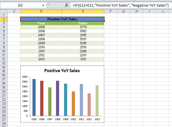
Enter any condition in the Linked Cell, now you should see the Chart title is changing as per the condition. The following screen-shot will show you how to do this.
Now you can see the conditional formula in the linked Cell which is reflecting in the Chart title.
Changing the Chart title based on Pivot Table Filtered Cell
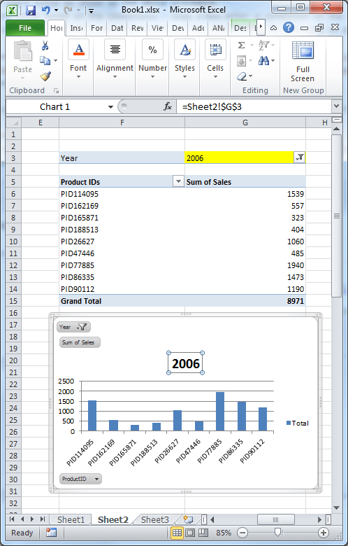
Same like above you can link a Pivot table filtered field cell to the chart title. Chart will change dynamically when you change filter of the pivot table. The following screen-shot will show you how to link a pivot table filter header to a chart title.
Her you can clearly observe that, chart title is linked to to the pivot table filtered cell. We have highlighted in the Yellow (G2), showing 2006 in the filter. You can see the same pivot table filtered value (2006) is showing as a chart title.



you have written a really good article,i found this very helpful….