LOOKUP Function in Excel – Formula Explained with Examples

LOOKUP Function: Explained with Examples

LOOKUP Formula is basic LookUp function in Excel, it is provided for backward compatibility. LookUp function is helpful if you want to look up a value in either in one-row or one-column data range or any array.

When we have array of values, and if you want to extract the result of a particular value from the data. We can use LookUp Formula to do this. Below is the pictorial representation of LOOKUP Formula.

Here we have List of Weekdays (Sunday to Saturday) and its IDs (1,2,…7). And we can specify the Lookup Value and Lookup Array in the Formula as show n below to lookup the respective value.

Here, A1:B7 is lookup-range and D4 is the lookup_value. And we will get the Wednesday as result for the lookup value(4).

What is the use of LOOKUP function?

LOOKUP Function in Excel returns a value from a table or from an array.

What is the syntax of LOOKUP function?

It has 2 different syntax:

• Syntax #1: LOOKUP(lookup_value, array): It is helpful when we have the single set of range of array with lookup vector.
• Syntax #2: LOOKUP(lookup_value, lookup_vector, result_vector): It is helpful when we have two different arrays one for lookup vectors and the other one for lookup arrays or range

• lookup_value: The value you want to look for
• array: The array of values that contain the value you want to look for
• lookup_vector: The range of cells that contains the value you want to look for
• result_vector: The range of cells that contains the value you want to return

Examples on LOOKUP Function in Excel

Syntax #1

LOOKUP function searches for the value in the first row or column of an array and returns the corresponding value in the last row or column of the array.

Example 1:

=LOOKUP(3,{1,2,3,4;”One”,”Two”,”Three”,”Four”})

Looks for 3 in the array and returns its corresponding value i.e; “Three”.

Example 2:
=LOOKUP(3,A5:B9)

Looks for lookup value (4) in the array (first column of the lookup range. i.e; A5:A9) and returns its corresponding value (right or second column of the lookup range. i.e; B5:B9).

Syntax #2

LOOKUP function searches for value in the lookup_range and returns the corresponding value in the result_range.

Example 3:
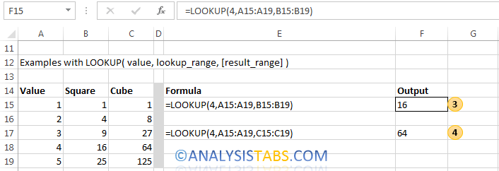
=LOOKUP(4,A15:A19,B15:B19)
Looks for 4 in the lookup range (first set of range in the formula i.e; A15:A19) and returns its corresponding value from the result range (second set of the range in the formula i.e; B15:B19)

Example 4:
=LOOKUP(4,A15:A19,C15:C19)

Looks for 4 in the lookup range (first set of range in the formula i.e; A15:A19)and returns its corresponding value from the result range (second set of the range in the formula i.e; C15:C19)

Reference:

Please refer the below article for more Lookup & Reference Excel functions.
Lookup & Reference Excel Formulas

Please refer the below article for more Excel Functions.
Excel Formulas | Home