Vlookup syntax and definition will help you to understand the syntax and definition of Vlookup formula in MS Excel 2007, 2010 and 2013. VLOOKUP function is used to search a value in the first column of a range of cells, and then return a respective value from any cell on the same row of the range. For example, assume that you have list of country names and its population and capital in a range A1:C200. Now if you want to look up the capital or population of a country, you can simply use vlookup function to quickly get the respective Capital and Population of the given country.
Vlookup Syntax and Definition
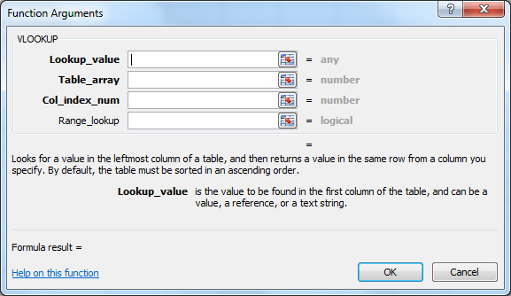
Following is the Vlookup Syntax in Microsoft Office Excel. Syntax of vlookup formula contains required four arguments or parameters to work in MS Excel.
VLOOKUP(lookup_value, table_array, col_index_num,
Here is the detailed explanation of arguments for Vlookup formula.
• lookup_value : lookup_value is the first parameter of excel Vlookup formula . lookup_value is a required parameter in Vlookup function in excel . Lookup value is a value which user wants to search in the first column of a range array and wants the respective row values to be returned. If excel finds lookup value in the table array it will return the respective row value of the given column in the range. Otherwise it will return #N/A error.
• table_array: table_array is the second parameter of excel Vlookup formula. table_array is a required parameter in Vlookup function in excel. table_array is a range in Excel worksheet which user wants to search the lookup value in the first column of this table array.
Note: Vlookup function is not a case sensitive.
• col_index_num: col_index_num is the third parameter of excel Vlookup formula. col_index_num is a required parameter in Vlookup function in excel. We need to mention column index number in the Vlookup formula to tell Excel from which column of the given array to be picked a row value of the lookup value. Column index number should be always greater than equals to 1 and less than or equals to number of columns in the given table array range. If you specify less than 1, Vlookup formula returns #VALUE error value. And if you mention a column number which is greater than number of columns in the lookup table array range, vlookup formula returns #Ref error value.
• range lookup : range_lookup is the fourth parameter of excel formula. range_lookup is an optional parameter in Vlookup function in Excel. Range lookup parameter is to specify whether user required an exact match values or an approximate match values. If you omit this parameter, Vlookup function treat it as TRUE as default.
You can mention TRUE (or 1) or FALSE (or 0) as a range lookup. Here TRUE searches for the exact match and returns the respective row values if match founds. Otherwise Vlookup returns approximate row values of the given lookup value. I.e. less than the exact match. Here TRUE and FALSE are Boolean values.
FALSE returns the Exact matched row values. If lookup value not found in the first column of the table array, vlookup function returns #N/A error value.
Vlookup Syntax and Examples
Following are the detailed explained examples of Vlookup syntax. We will take the same example explained in the beginning of this topic.
Explanation:
Example data to explain Vlookup Syntax
Here is the example data that is country in column A, population of the country in column B and capital of the country in column C. We are just taking random 10 countries and its capital and population information for our exercise.
Source: Wiki:VBA Programming
Here just build an environment where we can select the Country from the list of countries and we should see the respective Population and Capital City of the selected country.
Here is the example data which I have entered in the range A1 to C11 to explain Vlookup Syntax and Definition in Excel. You can see the table array “A1: C11” below
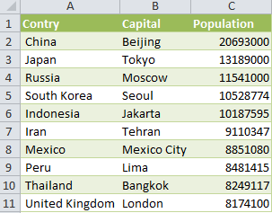
Sample Data: vlookup Syntax and Definition
And here is the environment which I want to prepare. User wants to select a country at A15 and the remaining fields (Capital, Population) should be populated automatically.
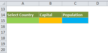
To Explain vlookup Syntax and Definition
We can do this using Vlookup function. Let us use Data Validation tool to provide a drop-down list at Range A15, and put a Vlookup formula to lookup the value in the table array range for the selected county and populate the Capital and Population of the Country at B15 and C15 respectively.
Here is the example screen-shot to explain putting a drop-down a Range A15.
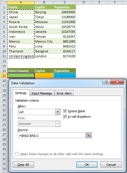
Providing drop-down list
• Select Range A15.
• Select Data Validation utility from the Data ribbon menu.
• Select the List in the allow drop-down and Range A2 to A11 in the Source drop-down list. And then select OK button.
Now you can see the drop-down at Range A15 as shown below.
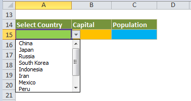
Drop-down in Range
Now place the below Vlookup formula at Range B15 and C15. Formula at B15 will return the second column from the table array. Formula at C15 will return the third column from the table array.
At B15 type this formula: =VLOOKUP(A15,A1:C11,2,FALSE)
At C15 type this formula: =VLOOKUP(A15,A1:C11,3,FALSE)
Now the environment looks as shown below:
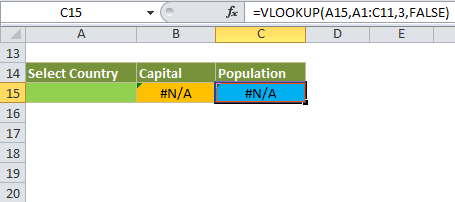
Vlookup formula in Range
Range A15 will have a drop-down list with countries.
Range B15 will have a vlookup formula which is mentioned above to get the City of the selected Country at A15.
Range C15 will have a vlookup formula which is mentioned above to get the Population of the selected Country at A15.
Now you can select any country at A15 and observe that respective Capital and City is populating at B15 and C15.
Explanation of Vlookup Syntax and formula in Cell
Let us see the formulas which we have used at B15 and C15.
Vlookup Syntax used at Range B15
Formula at B15 is “=VLOOKUP(A15,A1:C11,2,FALSE)”. We have used this Vlookup syntax to pull the Capital City that is 2nd Column in the Table array. Let us split the Syntax and see importance of each part of the Vlookup syntax (i.e. each parameters in the vlookup syntax).
A15: This is the lookup value and the first parameter in the Vlookup syntax. And we are using lookup value for to search the lookup value (i.e. country) in the first column of the table array range (i.e. Range A1:C15). Please note, vlookup is not a case sensitive, look up values can be in any case and it will return the first matched values in the table array. The data in the table array can be in any case. For Example, if you want to look for China in the table array, your lookup value can be china, CHINA, China, etc…, this will just look for the word and not a case sensitive.
A1:C11: This is the table array range and the second parameter in the vlookup function. Lookup value will be searched in the first column of the table array (i.e; A1:A15) and vlookup will return the respective matched row values as per the column index number. Most of the time we will lock the table array range, as we use table array in multiple cells by just dragging the vlookup formulas in the range. So that table arrange will not change. So use $A$1:$A$15, instead of just using A1:A15 in the vlookup syntax.
2: This the column index number and third parameter in the Vlookup syntax. This will tell Vlookup to return 2nd column values from the table array (B1:B15, i.e. Capital City). This you can provide as per the requirement. If you want Population, this should be 3, instead of 2. In real-time projects column index number of vlookup syntax will be depending on the table data range and the required field information to be returned. For example, if you have 50 columns in your data in the worksheet or any sheet in your workbook. And if you want to look up some data and fetch the data from those worksheets. You may use any number from 1 to 50. If you have 5o columns data, your column index should be any value between 1 and 50. And it should not be less than 1 and more than 50. You will see the error values if you provide wring column index numbers in the lookup syntax. You will see #VALUE error value if you enter column index number which is less than 1. And you will see #Ref error value, if you enter column index number which is more than number of columns in the table array range in your data sheet.
False: This the Boolean range lookup value and the fourth parameter in the vlookup syntax. This will tell vlookup function whether to look for exact match or approximate value in the first column of the table array. If you mention True, instead of False in vlookup formula. Vlookup will return values for approximate lookup value if not found the exact match. Most of the times we look for the exact values and use the FALSE as match index value.
Vlookup Syntax used at Range C15
Formula at C15 is “=VLOOKUP(A15,A1:C11,3,FALSE)”. We have used this Vlookup syntax to pull the Population that is 3nd Column in the Table array. Let us split the Syntax and see importance of each part of the Vlookup syntax (i.e. each parameters in the vlookup syntax).
A15: This is the lookup value and the first parameter in the Vlookup syntax. And we are using lookup value for to search the lookup value (i.e. Country) in the first column of the table array range (i.e. Range A1:C15, list of countries). Please note, vlookup is not a case sensitive, look up values can be in any case and it will return the first matched values in the table array. The data in the table array can be in any case. For Example, if you want to look for China in the table array, your lookup value can be china, CHINA, China, etc…, this will just look for the word and not a case sensitive.
A1:C11: This is the table array range and the second parameter in the vlookup function. Lookup value will be searched in the first column of the table array (i.e. A1:A15, list of countries) and vlookup will return the respective matched row values as per the column index number, in this case 3rd column. Most of the time we will lock the table array range, as we use table array in multiple cells by just dragging the vlookup formulas in the range. So that table arrange will not change. So use $A$1:$A$15, instead of just using A1:A15 in the vlookup syntax.
2: This the column index number and third parameter in the Vlookup syntax. This will tell Vlookup to return 3rd column values from the table array (C1:C15, i.e. Population of the country). This you can provide as per the requirement. If you want City, this should be 2, instead of 3. In real-time projects column index number of vlookup syntax will be depending on the table data range and the required field information to be returned. For example, if you have 50 columns in your data in the worksheet or any sheet in your workbook. And if you want to look up some data and fetch the data from those worksheets. You may use any number from 1 to 50. If you have 5o columns data, your column index should be any value between 1 and 50. And it should not be less than 1 and more than 50. You will see the error values if you provide wring column index numbers in the lookup syntax. You will see #VALUE error value if you enter column index number which is less than 1. And you will see #Ref error value, if you enter column index number which is more than number of columns in the table array range in your data sheet.
False: This the Boolean range lookup value and the fourth parameter in the vlookup syntax. This will tell vlookup function whether to look for exact match or approximate value in the first column of the table array. If you mention True, instead of False in vlookup formula. Vlookup will return values for approximate lookup value if not found the exact match. Most of the times we look for the exact values and use the FALSE as match index value.
Awesome! Thank you